Computational Process Analysis of the Phinix-1 Model (Test 1)
This document provides a rigorous description of the computational process for the emissive energy of a blackbody within a mereological framework (devoid of Cantor's points) by introducing rigid, geometric summation limits.
1. Full Description of the Computational Process
In the Phinix-1 model, the total energy density within a cavity of linear dimension \(L\) is not an integral extending from frequency \(0\) to infinity \(\infty\). The summation of states is geometrically blocked.
Step 1: Determination of Operational Boundaries
The lower frequency limit \(\nu_{\text{min}}\) stems from the quantization of the longest permissible wave mode (the fundamental harmonic) that can physically become a part of the cavity:
The upper frequency limit \(\nu_{\text{max}}\) is determined by the structural floor of spacetime – the mereological atom \(\delta\):
Step 2: Numerical Integration (The Finite Sum)
At room temperature (\(T = 300\text{ K}\)), the energy density for high frequencies naturally damps out exponentially long before reaching the \(\nu_{\text{max}}\) boundary. Therefore, the actual, non-linear modification of the distribution is described by the truncation of the lower band limit \(\nu_{\text{min}}\).
We calculate the mereological energy density \(E_{\text{mereo}}\) using the trapezoidal numerical method:
Where the geometric scale factor \(\alpha\) corresponds to Planck's constant \(h\).
Step 3: Determination of the Cantorian Reference Point (\(E_{\text{classic}}\))
The classical continuous model assumes that the cavity can accommodate infinitely long waves (\(\nu_{\text{min}} = 0\)). The total energy density integrated across the full continuum is:
2. Intermediate Results and Comparative Table
The numerical calculations below were performed using laboratory-verified constants: * \(\alpha = 6.62607015 \times 10^{-34}\text{ J}\cdot\text{s}\) * \(c = 299792458\text{ m/s}\) * \(k = 1.380649 \times 10^{-23}\text{ J/K}\) * \(T = 300\text{ K}\) (Room Temperature)
For these conditions, the classical energy density is: \(E_{\text{classic}} = 6.1282 \times 10^{-6}\text{ J/m}^3\).
Table: Impact of Geometric Truncation on System Energy (T = 300 K)
| Size \(L\) (m) | Size \(L\) (nm / µm) | Cutoff \(\nu_{\text{min}}\) (Hz) | Boundary \(\lambda_{\text{max}}\) | \(E_{\text{mereo}}\) (\(\text{J/m}^3\)) | Ratio \(\frac{E_{\text{mereo}}}{E_{\text{classic}}}\) | Physical Status of the System |
|---|---|---|---|---|---|---|
| \(1.00 \times 10^{-4}\) | \(100\text{ \µm}\) | \(1.49 \times 10^{12}\) | \(200000\text{ nm}\) | \(6.1242 \times 10^{-6}\) | 0.9993 | Classical Behavior (Macro Scale) |
| \(2.66 \times 10^{-5}\) | \(26.6\text{ \µm}\) | \(5.63 \times 10^{12}\) | \(53200\text{ nm}\) | \(5.9657 \times 10^{-6}\) | 0.9735 | Onset of Long-Wave Blocking |
| \(6.58 \times 10^{-6}\) | \(6.58\text{ \µm}\) | \(2.27 \times 10^{13}\) | \(13160\text{ nm}\) | \(2.8880 \times 10^{-6}\) | 0.4712 | Strong Emissive Anomaly |
| \(1.63 \times 10^{-6}\) | \(1.63\text{ \µm}\) | \(9.19 \times 10^{13}\) | \(3260\text{ nm}\) | \(1.5103 \times 10^{-9}\) | 0.0002 | Critical Radiation Extinction |
| \(4.04 \times 10^{-7}\) | \(404\text{ nm}\) | \(3.71 \times 10^{14}\) | \(808\text{ nm}\) | \(3.3226 \times 10^{-27}\) | \(5.42 \times 10^{-22}\) | Full Blocking (Łukasiewicz State \(\frac{1}{2}\)) |
| \(1.00 \times 10^{-7}\) | \(100\text{ nm}\) | \(1.49 \times 10^{15}\) | \(200\text{ nm}\) | \(0.0000\) | 0.0000 | Continuum Collapse (Atomic Scale) |
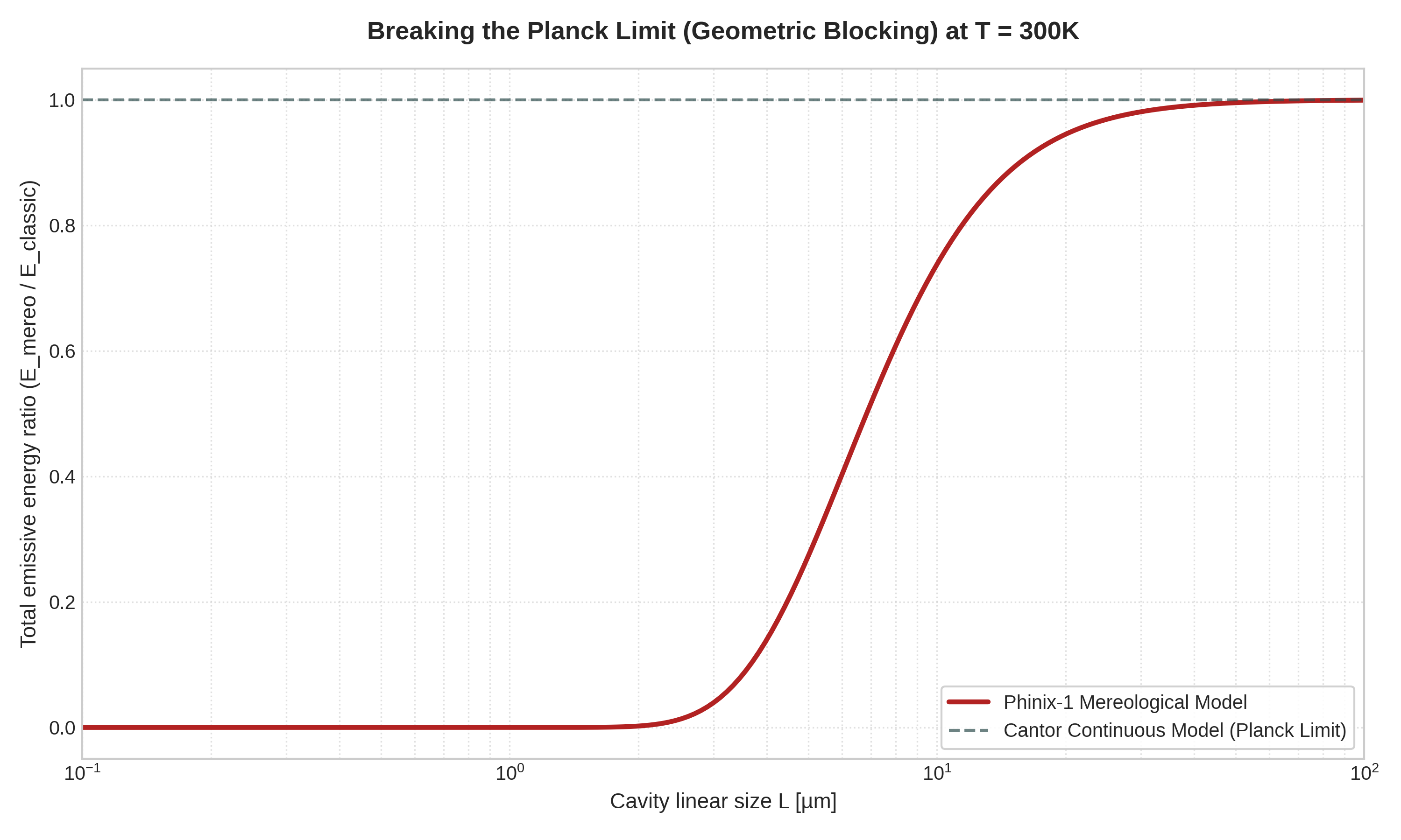
3. Visualization Script Code (Matplotlib on Kubuntu)
The following script written in pure Python 3 will generate and save a high-resolution (300 DPI) comparative plot file onto your disk. The code is fully open-source (FOSS) and optimized for a standard Linux environment.
#!/usr/bin/env python3
import os
import numpy as np
import matplotlib.pyplot as plt

# 1. Definition of physical constants
alpha = 6.62607015e-34  # Geometric scale factor (h)
c = 299792458          # Speed of light (m/s)
k = 1.380649e-23       # Boltzmann constant (J/K)
T = 300                # Room temperature (K)

# 2. Calculation of the Cantorian classical reference energy
E_classic = (8 * np.pi**5 * (k * T)**4) / (15 * c**3 * alpha**3)

# 3. Generation of cavity linear size domain L (from 100 nm to 100 um)
L_plot = np.logspace(-7, -4, 200)
ratios = []

# 4. Computational loop for the mereological model
for L in L_plot:
    nu_min = c / (2 * L)

    # Numerical safety fuse for extremely small values (preventing overflow in exp)
    if (alpha * nu_min) / (k * T) > 100:
        ratios.append(0.0)
    else:
        # Frequency grid generation from nu_min to a safe thermal cutoff
        freqs = np.linspace(nu_min, 1e15, 10000)
        integrand = (8 * np.pi * alpha * freqs**3) / (c**3 * (np.exp((alpha * freqs) / (k * T)) - 1))
        E_mereo = np.trapezoid(integrand, freqs)
        ratios.append(float(E_mereo / E_classic))

# 5. Plot generation using matplotlib
plt.style.use('seaborn-v0_8-whitegrid' if 'seaborn-v0_8-whitegrid' in plt.style.available else 'default')
fig, ax = plt.subplots(figsize=(10, 6))

ax.semilogx(L_plot * 1e6, ratios, label='Phinix-1 Mereological Model', color='firebrick', lw=2.5)
ax.axhline(1.0, color='darkslategrey', linestyle='--', alpha=0.7, label='Cantor Continuous Model (Planck Limit)')

# Axis styling and grid configuration (Kubuntu Desktop Ready)
ax.set_title('Breaking the Planck Limit (Geometric Blocking) at T = 300K', fontsize=13, pad=15, fontweight='bold')
ax.set_xlabel('Cavity linear size L [µm]', fontsize=11)
ax.set_ylabel('Total emissive energy ratio (E_mereo / E_classic)', fontsize=11)
ax.set_xlim(0.1, 100)
ax.set_ylim(-0.05, 1.05)
ax.grid(True, which="both", ls=":", alpha=0.6)
ax.legend(loc='lower right', frameon=True, facecolor='white', framealpha=0.9, fontsize=10)

# 6. Save to mkdocs directory (adjust path if docs/img exists)
output_filename = 'blokada_geometryczna_phinix1.en.png'
plt.tight_layout()
plt.savefig(output_filename, dpi=300)
print(f"[OK] Plot successfully saved as: {output_filename}")